[Paper Review] DDIM

Denoising Diffusion Implict Models(DDIM) 논문 리뷰

논문 링크 arxiv

DDPM은 높은 퀄리티의 이미지 생성을 이루어냈다. 하지만 sampling 과정에서 여러 step을 거쳐 Markov chain을 시뮬레이션하기 때문에, 시간이 많이 걸린다는 단점이 있다. 이 논문에서는 sampling 과정을 가속화하는 Denoising Diffusion Implicit Models(DDIM)을 제안한다.

Introduction

DDPM이나 NCSN과 같은 iterative generative models은 높은 품질의 sample을 생성하기 위해서는 많은 iteration을 필요로 한다는 단점이 있다. DDPM의 경우, foward diffusion process(data to noise)의 역을 근사화하여 generative process를 만들었으며, sample 하나당 수천의 step을 거친다. 이는 Network를 한번만 통과하면 되는 GAN에 비해 엄청난 시간이 소요된다.

nvidia 2080 ti GPU로 32*32 이미지 500,000장을 sampling할때 소요되는 시간은 DDPM은 약 20시간, GAN은 1분도 채 걸리지 않는다고 한다. 같은 조건에서 해상도만 256*256으로 변경할 경우, DDPM은 거의 1000시간 가까이 걸린다고 한다.

논문에서는 DDPM의 train method는 그대로 사용하면서, DDPM처럼 Markovian process를 사용하는 대신, non-Markovian으로 일반화하여 빠른 sampling을 하는 방법을 제안한다

Background

DDIM의 베이스가 되는 DDPM을 다시 살펴보자.

data의 분포 $q(x_0)$가 주어졌을 때, 이를 근사화하는 network인 $p_\theta(x_0)$를 학습해야한다.

\[p_\theta(x_0) = \int p_\theta(x_{0:T})dx_{1:T} \;\;\;\;\;\ p_\theta(x_{0:T}) := p_\theta(x_T)\prod_{t=1}^{T}p_\theta ^{(t)} (x_{t-1}|x_t) \tag{1}\]

ELBO를 사용하여 $p_\theta(x_0)$에 대한 object function을 다음과 같이 도출할 수 있다.

\[\underset{\theta}{max}\; \mathbb{E}_{q(x_0)}[\log p_\theta(x_0)] \leq \underset{\theta}{max}\; \mathbb{E}_{q(x_0, x_1, \cdots, x_T)} [\log p_\theta(x_{0:T}) - \log q(x_{1:T}|x_0)] \tag{2}\]

또한 감소하는 값인 $\alpha_{1:T}$($1-\beta$)를 파라미터화한 Markov chain을 통해 foward process를 다음과 같이 $x_0$와 noise 변수인 $\epsilon$을 이용해 표현할 수 있다.

\[\begin{align} q(x_t|x_0) &:= \int q(x_{1:t}|x_0)dx_{1:t-1} = N(x_t;\sqrt{\alpha_t}x_0, (1-\alpha_t)I) \nonumber \\ x_t &= \sqrt{\alpha_t}x_0 + \sqrt{1-\alpha_t}\epsilon \;\;\;\;\;\;\;\epsilon \sim N(0, I)\tag{4} \end{align}\]

mean function이 학습 가능하고, 고정된 variance를 가진 Gaussian으로 가정한다면, Eq (2)는 다음과 같이 simplify 할 수 있다.

\[L_\gamma (\epsilon_\theta) := \sum_{t=1}^{T} \gamma_t \mathbb{E}_{x_0 \sim q(x_0), \epsilon_t \sim N(0, I)} \left [\left| \left| \epsilon_\theta ^t (\sqrt{\alpha_t}x_0 + \sqrt{1-\alpha}\epsilon_t) - \epsilon_t\right| \right |^2_2 \right] \tag{5}\]

$\epsilon_\theta ^t$는 파라미터 $\theta^{t}$에 대한 함수이며 $\gamma _t$는 $\alpha_{1:T}$에 따라 달라지는 벡터이다. DDPM에서는 $\gamma$를 1로 고정시켰을 때 generation performance가 가장 좋다고 하였다.

DDPM에서 step의 길이 $T$는 가장 중요한 hyperparameter이다. $T$가 클때 reverse process는 Gaussian에 가까워지며, generative process의 성능이 좋아진다고 하며 $T=1000$과 같은 큰 값을 권장한다.

하지만, sample $x_0$을 얻기 위하여 $T$ step을 순차적으로 거쳐야하므로 DDPM의 sampling은 타 모델보다 훨씬 느리다.

Variational Inference for Non-Markovian Foward Process

논문에서는 많은 step을 필요로 하는 DDPM의 reverse process 대신, non-Markovian을 inference process로 사용하는 것을 제안한다.

3.1 Non-Markovian Foward process

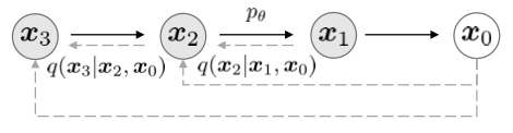
위 그림은 다음과 같이 수식으로 나타낼 수 있다.

\[q_\sigma(x_{1:T}|x_0) = q_\sigma (x_T | x_0)\prod_{t=2}^T q_\sigma (x_{t-1}|x_t, x_0) \\ \text{where}\;\;\;\;\;\; q_\sigma(x_T|x_0) = N(\sqrt{\alpha_T}x_0, (1-\alpha_T)I) \tag{6}\]

DDPM의 foward process 수식인 $q(x_{1:T}|x_0) = \prod_{t=1}^{T}q(x_t|x_{t-1})$과 다른점은 오른쪽 수식에 $x_0$가 포함된다는 것이다.

즉, DDPM은 $x_t$가 바로 이전 step인 $x_{t-1}$에 의해서만 결정되는 Markovian인 반면, DDIM은 $x_{t-1}$과 $x_0$에 의해 결정되는 Non-Markovian이다.

모든 $t>1$에 대해

\[q_\sigma(x_{t-1}|x_t, x_0) = N\left(\sqrt{\alpha_{t-1}}x_0 + \sqrt{1-\alpha_{t-1}-\sigma_t^2} \cdot \frac{x_t-\sqrt{\alpha_t}x_0}{\sqrt{1-\alpha_t}}, \sigma_t^2 I \right) \tag{7}\]

위 mean function은 모든 $t$에 대한 $q_\sigma(x_t|x_0) = N(\sqrt{\alpha_t}x_0, (1-\alpha_t)I)$를 보장한다. 이는 주변 distribution과 일치하는 inference joint distribution을 정의한다.

또한 $\sigma$ 값은 forward process가 얼마나 stochastic한지 조절한다. 0에 가까워질수록 stochastic하지않고 fix된다.

Bayes’s rule에 의해 $q_\sigma (x_{t}|x_{t-1}, x_0)$는 다음과 같이 나타낼 수 있다.

\[q_\sigma (x_{t}|x_{t-1}, x_0) = \frac{q_\sigma (x_{t-1}|x_t, x_0) q_\sigma (x_{t}|x_0) }{q_\sigma (x_{t-1}|x_0) }\]

즉 Eq 6.을 다시 쓰면 다음과 같다.

\[\begin{align} q_\sigma(x_{1:T}|x_0) &= \prod_{t=1}^T q_\sigma(x_t|x_{t-1}, x_0) \nonumber \\ &= q_\sigma(x_1|x_0)\times \frac{q_\sigma(x_1|x_2, x_0)q_\sigma(x_2|x_0)}{q_\sigma(x_1|x_0)} \times\frac{q_\sigma(x_2|x_3, x_0)q_\sigma(x_3|x_0)}{q_\sigma(x_2|x_0)} \times \cdots \times \frac{q_\sigma(x_{T-1}|x_T, x_0)q_\sigma(x_T|x_0)}{q_\sigma(x_{T-1}|x_0)} \nonumber \\ &= q_\sigma(x_T|x_0)\prod_{t=2}^T q(x_{t-1}|x_t,x_0) \nonumber \end{align}\]

3.2 Generative process and Unified Variational Inference objective

이 부분에는 generative process $p_\theta(x_{0:T})$를 정의한다. 각 step $p_\theta^{(t)}$는 foward process의 $q_\sigma(x_{t-1}|x_t, x_0)$를 이용한다.

noise $x_t$가 주어지면, 이를 활용하여 $x_0$를 예측하고, $x_t$와 $x_0$를 이용하여 $q_\sigma(x_{t-1}|x_t, x_0)$로 $x_{t-1}$을 sampling한다.

$\epsilon_\theta^{(t)}(x_t)$는 $x_0$없이 $x_t$를 이용해 $\epsilon_t$를 예측한다. Eq 4.를 재작성하여 $x_t$를 이용하여 $x_0$을 예측하는 denoised observation을 얻을 수 있다.

\[f_\theta^{(t)}(x_t) := \frac{x_t - \sqrt{1-\alpha_t}\cdot\epsilon_\theta^{(t)}(x_t)}{\sqrt{\alpha_t}} \tag{9}\]

Eq 7.에서 $x_0$를 $f_\theta^{(t)}(x_t)$로 대체한 $q_\sigma (x_{t-1}|x_t, f_\theta^{(t)}(x_t))$를 이용해 다음과 같이 generative process를 정의할 수 있다.

\[p_\theta^{(t)}(x_{t-1}|x_t) = \begin{cases} N(f_\theta^{(1)}(x_1), \sigma_1^2I) & \text{ if } t=1 \\ q_\sigma(x_{t-1}|x_t, f_\theta^{(t)}(x_t)) & \text{ otherwise,} \end{cases} \tag{10}\]

이말은 예측한 $epsilon_t$와 $x_t$를 이용하여 $x_0$를 예측하고, 이 $x_0$, $x_t$를 이용해 $x_{t-1}$을 예측할 수 있다는 것을 의미한다.

$\epsilon_\theta$에 대한 함수인 variational inference objective를 통해 $\theta$를 최적화할 수 있다.

\[\begin{align} J_\sigma(\epsilon_\theta) :&= \mathbb{E}_{x_{0:T}\sim q_\sigma(x_{0:T})} [\log q_\sigma(x_{1:T}|x_0)-\log p_\theta(x_{0:T})] \nonumber\\ &= \mathbb{E}_{x_{0:T}\sim q_\sigma(x_{0:T})}\left[\log \left(q_\sigma (x_T | x_0)\prod_{t=2}^T q_\sigma (x_{t-1}|x_t, x_0) \right) - \log \left( p_\theta(x_T)\prod_{t=1}^{T}p_\theta ^{(t)} (x_{t-1}|x_t)\right) \right] \nonumber \\ &= \mathbb{E}_{x_{0:T}\sim q_\sigma(x_{0:T})} \left[\log q_\sigma(x_T|x_0)+\sum_{t=2}^T \log q_\sigma(x_{t-1}|x_t, x_0) - \sum_{t=1}^{T}\log p_\theta^{(t)}(x_{t-1}|x_t) - \log p_\theta(x_{T}) \right] \nonumber \\ \tag{11} \end{align}\]

위 식에서 $q_\sigma (x_{1:T}|x_0)$은 Eq 6.에서, $p_\theta(x_{0:T})$은 Eq 1.로 치환하였다.

$J_\sigma(\epsilon_\theta)$을 보면 $\sigma$값에 따라 다른 variational objective으로 다른 모델을 학습시켜야 함을 알 수 있다. 하지만, 다음 이론이 성립한다.

Theorem 1. $\sigma > 0$일 때 $J_\sigma = L_\gamma + C$를 만족하는 $\gamma \in \mathbb{R}_{>0}^T$과 $C \in \mathbb{R}$이 존재한다.

즉, $\gamma$이 어떤 값에서는 $L_\gamma = J_\sigma$를 성립한다는 것을 알 수 있다.

Variational object $L_\gamma$는 $\epsilon_\theta^{(t)}$가 다른 $t$와 공유하지 않을때 이 $\epsilon_\theta^{(t)}$에 대한 최적해는 $\gamma$와 상관이 없다. 이로써 다음과 같은 2가지 특성을 알 수있다.

     1. DDPM의 variational lower bound에 대한 object function으로 $L_1$을 사용할 수 있다.

    2. $J_\sigma$가 Theorem 1에서 $L_\gamma$의 일부와 동일하기 때문에. $J_\sigma$의 최적해는 $L_1$과 동일하다.

Theorem 1 부록

$$ \begin{aligned} J_\sigma (\epsilon_\theta) & \equiv \mathbb{E}_{x_{0:T} \sim q_\sigma (x_{0:T})} \bigg[ \log q_\sigma (x_T | x_0) + \sum_{t=2}^T \log q_\sigma (x_{t-1} | x_t, x_0) - \sum_{t=1}^T \log p_\theta^{(t)} (x_{t-1} | x_t) \bigg] \\ & \equiv \mathbb{E}_{x_{0:T} \sim q_\sigma (x_{0:T})} \bigg[ \sum_{t=2}^T \log \frac{q_\sigma (x_{t-1} | x_t, x_0)}{p_\theta^{(t)} (x_{t-1} | x_t)} - \log p_\theta^{(1)} (x_0 | x_1) \bigg] \\ &= \mathbb{E}_{x_{0:T} \sim q_\sigma (x_{0:T})} \bigg[ \sum_{t=2}^T D_{KL} (q_\sigma (x_{t-1} | x_t, x_0) || p_\theta^{(t)} (x_{t-1} | x_t)) - \log p_\theta^{(1)} (x_0 | x_1) \bigg] \\ \end{aligned} $$ $\equiv$라는 기호는 $\epsilon_\theta$과 상관없는지만 $q\_\sigma$에 영향을 받는 값과 같다는 것을 나타낸다. $t>1$일 때, $d$는 $x_0$의 차원이며 $$ \begin{aligned} & \mathbb{E}_{x_0, x_t \sim q_\sigma (x_0, x_t)} [D_{KL} (q_\sigma (x_{t-1} | x_t, x_0) || p_\theta^{(t)} (x_{t-1} | x_t))] \\ &= \mathbb{E}_{x_0, x_t \sim q_\sigma (x_0, x_t)} [D_{KL} (q_\sigma (x_{t-1} | x_t, x_0) || q_\sigma (x_{t-1} | x_t, f_\theta^{(t)}(x_t)))] \\ & \equiv \mathbb{E}_{x_0, x_t \sim q_\sigma (x_0, x_t)} \bigg[ \frac{\| x_0 - f_\theta^{(t)} (x_t) \|_2^2}{2\sigma_t^2} \bigg] \\ &= \mathbb{E}_{x_0 \sim q(x_0), \epsilon \sim \mathcal{N}(\textbf{0},I), x_t=\sqrt{\alpha_t}x_0 + \sqrt{1-\alpha_t} \epsilon} \bigg[ \frac{ \bigg\| \frac{x_t - \sqrt{1-\alpha_t}\epsilon}{\sqrt{\alpha_t}} - \frac{x_t - \sqrt{1-\alpha_t} \epsilon_\theta^{(t)}(x_t)}{\sqrt{\alpha_t}} \bigg\|_2^2}{2\sigma_t^2} \bigg] \\ &= \mathbb{E}_{x_0 \sim q(x_0), \epsilon \sim \mathcal{N}(\textbf{0},I), x_t=\sqrt{\alpha_t}x_0 + \sqrt{1-\alpha_t} \epsilon} \bigg[ \frac{ \| \epsilon - \epsilon_\theta^{(t)} (x_t) \|_2^2}{2d \sigma_t^2 \alpha_t} \bigg] \\ \end{aligned} $$ $t = 1$일 때, $$ \begin{aligned} & \mathbb{E}_{x_0, x_1 \sim q_\sigma (x_0, x_1)} \bigg[ -\log p_\theta^{(1)} (x_0 | x_1) \bigg] \equiv \mathbb{E}_{x_0, x_1 \sim q_\sigma (x_0, x_1)} \bigg[ \frac{\| x_0 - f_\theta^{(1)} (x_1) \|_2^2}{2\sigma_1^2} \bigg] \\ = \; & \mathbb{E}_{x_0 \sim q(x_0), \epsilon \sim \mathcal{N}(\textbf{0},I), x_1=\sqrt{\alpha_1}x_0 + \sqrt{1-\alpha_1} \epsilon} \bigg[ \frac{ \| \epsilon - \epsilon_\theta^{(1)} (x_1) \|_2^2}{2d \sigma_1^2 \alpha_1} \bigg] \\ \end{aligned} $$ 따라서, 모든 $t \in \{1,\cdots,T\}$에 대하여 $\gamma_t = 1/(2d \sigma_t^2 \alpha_t)$일때, 모든 $\epsilon_\theta$에 대하여 $$ \begin{equation} J_\sigma (\epsilon_\theta) \equiv \sum_{t=1}^T \frac{1}{2d \sigma_t^2 \alpha_t} \mathbb{E} \bigg[ \| \epsilon_\theta^{(t)} (x_t) - \epsilon_t \|_2^2 \bigg] = L_\gamma (\epsilon_\theta) \end{equation} \nonumber $$ 이다. "$\equiv$"의 정의에 따라 $J_\sigma = L_\gamma + C$이다.

Sampling from Generalized Generative Process

objective funcition으로 $L_1$을 사용하여 DDPM의 Markovian process 뿐만 아니라, 이번 논문에서 제안하는 Non-Markovian process에 대한 generative process를 학습할 수 있다. stochastic의 정도를 나타내는 $\sigma$값을 조절하여 더 나은 sample을 생성하는 process를 찾을 수 있다.

4.1 Denoising Diffusion Implicit Models

Eq. 10의 $p_\theta (x_{1:T})$를 통해 $x_t$로부터 $x_{t-1}$를 생성할 수 있다.

\[x_{t-1} = \sqrt{\alpha_{t-1}} \underbrace{\left(\frac{x_t - \sqrt{1-\alpha_t}\epsilon_\theta^{(t)}(x_t)}{\sqrt{\alpha_t}} \right)}_{\text{예측된}x_0} + \underbrace{\sqrt{1 - \alpha_{t-1} - \sigma_t^2} \cdot \epsilon_\theta^{(t)}(x_t)}_{\text{direction pointing to }x_t} + \underbrace{\sigma_t\epsilon_t}_{\text{random noise}} \tag{12}\]

$\epsilon_t \sim N(0, I)$은 $x_t$와 무관한 표준 Gaussian noise이며 $\alpha_0 := 1$로 정의한다. 동일한 모델 $\epsilon_\theta$의 $\sigma$값을 조절함에 따라 generative process의 결과가 달라지므로 모델을 다시 학습할 필요가 없어진다. 모든 $t$에 대해 $\sigma_t = \sqrt{\frac{1-\alpha_{t-1}}{1-\alpha_t}}\sqrt{1 - \frac{\alpha_t}{\alpha_{t-1}}}$일때, foward process는 Markovian의 성질을 띄며 DDPM이 된다.

모든$t$에 대해 $\sigma_t = 0$일때, foward process는 주어진 $x_0$와 $x_{t-1}$에 의해 deterministic해진다.

    → DDIM이 됨, $t=1$에서는 제외

결과적으로 만들어진 모델은 $x_T$ ~ $x_0$의 latent variable에서 sample이 생성되는 implicit probabilistic model이 된다. 논문에서는 이 모델이 더이상 diffusion스럽지 않지만, DDPM의 object function을 따르기 때문에 Diffusion Implicit Probabilistic Model이라 명명한다고 한다.

4.2 Accreted Generation Processes

지금까지 generative process는 reverse process의 근사치로 간주되었다. foward process가 $T$ step을 가지고 있다면, generative process 역시 $T$ step을 sampling해야한다. 하지만 $q_\sigma (x_t|x_0)$가 고정되어있을 때 denoting objective $L_1$은 특정 foward process에 의존하지 않는다. 이때문에, $T$보다 작은 generative process를 고려할 수 있었다고 논문은 말한다.

foward process를 $x_{1:T}$가 아니라 부분집합 ${x_{\tau_1}, \cdots, x_{\tau_S}}$에 대해 정의할 수 있다. 이때 $\tau$는 길이가 $S$인 $[1, \cdots, T]$의 증가하는 부분 수열이다. $x_{\tau_1}, \cdots, x_{\tau_S}$에 대한 sequential forward process를 정의하여 $q(x_{\tau_i}| x_0) = N(\sqrt{\alpha_{\tau_i}}x_0, (1-\alpha_{\tau_i})I)$가 그림 2처럼 주변분포와 일치하도록 한다.

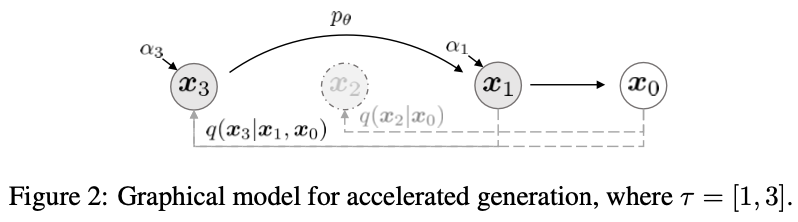
Generative process는 reversed($\tau$)에 따른 latent variables로 sampling되고, 이걸 sampling trajectory 라고 부른다. sampling trajectory의 길이가 $T$보다 작을수록 계산 효율성이 증가한다고 한다.

모델을 train할 때에는 DDIM 방식인 임의의 step에서 모델을 train하는것 보다 DDPM 방식인 수많은 step에 대해서 모델을 학습시키는게 더 효과적이다. 따라서 최근에는 DDPM으로 train한 다음, DDIM으로 sampling하는 경우가 많다고 한다.

4.3 Relevance to Neural ODEs

Eq. 12에 따라 DDIM 식($\sigma_t = 0$)을 다시 쓸수 있으며, 상미분 방정식(ODE)을 풀기 위한 Euler 적분과 유사해진다.

\[\frac{x_{t-\Delta t}}{\sqrt{\alpha_{t-\Delta t}}} = \frac{x_t}{\sqrt{\alpha_t}} + \left(\sqrt{\frac{1-\alpha_{t-\Delta t}}{\alpha_{t-\Delta t}}} - \sqrt{\frac{1-\alpha_t}{\alpha_t}} \right)\epsilon_\theta^{(t)}(x_t) \tag{13}\]

$\sqrt{\frac{1-\alpha}{\alpha}}$를 $\sigma$로, $\frac{x}{\sqrt{\alpha}}$를 $\overline{x}$로 reparameterize하여 Eq. 13은 다음 ODE를 통해 Euler 방법으로 처리할 수 있다.

\[d\;\overline{x}(t) = \epsilon_\theta ^{(t)} \left(\frac{\overline{x}(t)}{\sqrt{\sigma^2 + 1}} \right)d\;\sigma(t) \tag{14}\]

초기 조건은 $x(T) \sim N(0, \sigma(T))$이다. 이는 충분한 discretization step을 거치면 위 Eq. 14의 ODE를 reverse하여 generative process의 역인 encoding($x_0$ to $x_T$)이 가능함을 시사한다.

Experiments

이 section에서는 DDIM이 DDPM보다 generative process의 속도가 10배에서 100배까지 더 빨라짐을 보여준다. 게다가 초기 latent variables $x_T$가 고정되었을때, DDIM은 generation trajectory와 관계없이 high-level 이미지 feature를 유지하며 latent space에서의 직접적인 interpolation이 가능하다.

또한 DDIM은 sample을 encoding에 활용할 수 있으며 latent code에서 이미지의 reconstruction도 가능하다. 이는 stochastic sampling process인 DDPM은 할 수 없다.

각 데이터셋에서 $L_1$을 objective로 사용하고 $T=1000$으로 학습된 같은 모델을 사용하였다.

다른점은 모델에서 sampling 방법만 변화를 주었다. sampling속도를 제어하는 $\tau$와 모델이 얼마나 deterministic해지는지 결정하는 $\sigma$ 값을 조절한다.

여기서는 $[1, \cdots , T]$의 다른 부분 수열 $\tau$ 와 $\tau$의 요소로 구성된 variance hyperparameter인 $\sigma$를 사용한다 . 비교를 단순화하기 위해 $\sigma$를 4.1에서 언급했던 형태로 취할 수 있다.

\[\sigma_{\tau_i}(\eta) = \eta\sqrt{\frac{1-\alpha_{\tau_{i-1}}}{1-\alpha_{\tau_{i}}}}\sqrt{1 - \frac{\alpha_{\tau_{i}}}{\alpha_{\tau_{i-1}}}} \tag{16}\]

        ●$\eta = 1$ → DDPM

        ●$\eta = 0$ → DDIM

DDIM은 20~100 step 이내에 1000 step DDPM 모델과 비슷한 품질의 sample을 생성할 수 있다. 이는 기존 DDPM에 비해 10배에서 50배까지 빨라진 속도이다. CelebA 데이터셋에서 100 step DDPM의 FID는 20 step DDIM과 비슷하다.