[Paper Review] PromptStyler

PromptStyler 논문 리뷰

제목 : PromptStyler: Prompt-driven Style Generation for Source-free Domain Generalization

저자 : Junhyeong Cho, Gilhyun Nam, Sungyeon Kim, Hunmin Yang, Suha Kwak

링크 : arXiv Project Page

Vision-Language 공간(space)에서 두 모달리티 간의 전이성(transferability)이 존재한다는 것이 최근 연구를 통해 발견되었다. 이 논문은 이미지를 사용하지 않고, 오직 prompt만 사용하여 Style 변환을 수행하는 PromptStyler를 제안한다. 이는 pseudo-words(의사 단어)를 Styler word vector로 표현한 후, Space의 분포 변화를 시뮬레이션하여 다양한 스타일을 생성할 수 있다. 저자들은 이를 통해 이미지 학습 없이 다양한 데이터셋에서 Style 변환을 이루었다고 말한다.

Introduction

Domain Adaptation은 Train, Test 데이터 간의 분포 변화가 클 때(distribution shifts), target domain에 모델을 적응시켜 성능을 높인다. 하지만 완전히 새로운 domain에 대해서는 성능이 감소하기 때문에, Domain Generalization이라는 다양한 domain에 대해 모델을 일반화하는 연구가 진행되고 있지만 여러 한계에 부딫힌다.

논문에서는 “source domain 데이터 없이 모델의 latent space에서 다양한 분포 변화를 시뮬레이션하여 Domain Generalization를 효과적으로 수행할 수 있을지?“에 대한 질문을 던진다.

이 논문에서는 Large-scale Vision Language 모델에서 text가 joint vision-language space에서 관련 image를 대표할 수 있다는 점을 활용한다. 특히, cross-modal 전이 가능성을 보여준다.

cross-modal 전이

이 논문에서는 text feature로 Classifier를 train하고 image feature를 사용해 Classifier에서 inference하는 것을 말함.

이 train process를 통해 source-free Domain Generalization을 수행할 수 있으며, image 없이 prompt(text)만을 통하여 다양한 분포 변화를 시뮬레이션 할 수 있다.

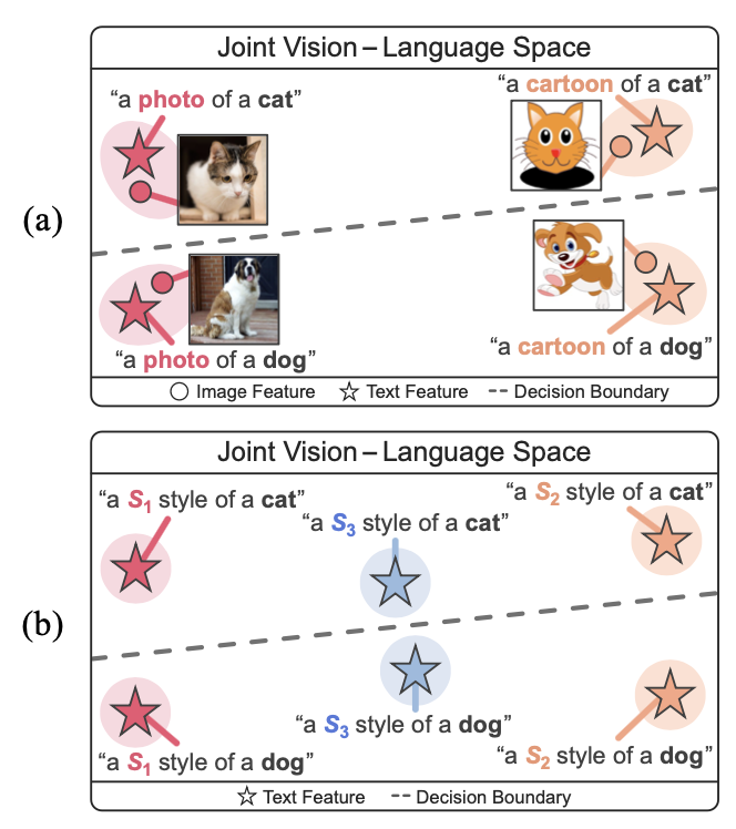
저자들은 learnable한 단어 vector를 통해 다양한 style을 합성할 수 있는 prompt 기반 Style 생성 기법인 PromptStyler를 제안한다.

OpenAI에서 개발한 Vision-Language 모델 CLIP을 사용하여 pseudoword $\mathit{S}_{\boldsymbol{\ast}}$에 대한 word vector(“a painting in the style of $\mathit{S}_{\boldsymbol{\ast}}$”)로 스타일을 포착할 수 있다고 한다.

PropmtStyler는 다음과 같은 특성이 있다.

1. orthogonal style features : style feature들이 서로 영향을 주지 않으면서 독립적으로 구별될 수 있는 것
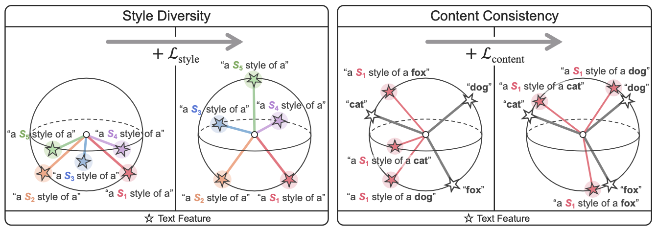
   • style diversity(다양성)를 최대화
2. content consistency : 학습된 style이 정보를 왜곡하는 것을 방지
   • style-content feature는 content prompt(“[class]”)로부터 얻은 content feature가 다른 feature들 보다 더 가까이 위치하도록 강제
   • style-contents feature는 style-content prompt(“a $\mathit{S}_{\boldsymbol{\ast}}$ style of a [class]”)에서 얻어짐

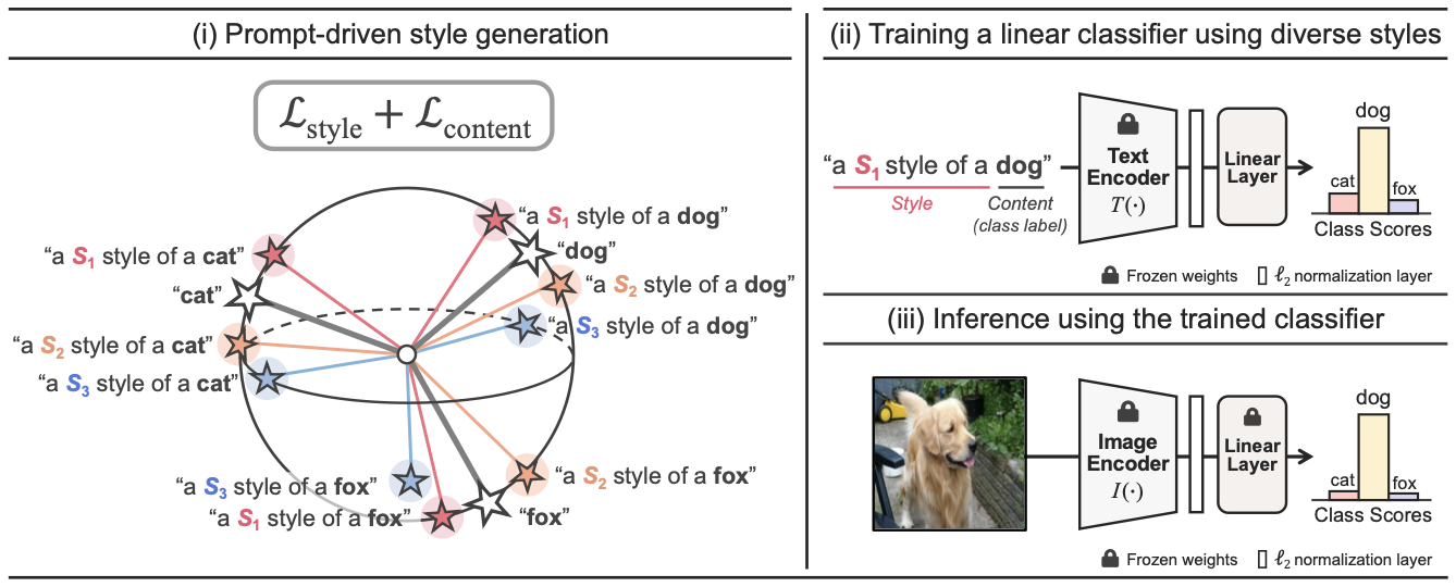
학습된 style word vector는 style-content feature를 합성하여 Classifier를 Train시킨다. 이 feature은 joint space에서 “알고있는” content 이미지를 “알려지지 않은” style로 시뮬레이션할 수 있다.

Linear Classifier은 [style-content feature, content(“[class]”)] 쌍 데이터로 학습된다.

[style-content feature, content(“[class]”)] == [input, label]

inference 절차는 다음과 같다.

1. Image Encoder가 Input 이미지에서 feature 추출
2. 추출된 feature를 학습된 Classifier에 입력

Pretrained Vision-Language 모델에서 사용한 Text/Image Encoder를 사용.

Text Encoder는 Train, Image Encoder는 Inference에 사용

논문에서 제안한 모델은 CLIP에 비해 경량화 되었지만, 더 빠른 Inference 속도를 보여줬다고 말한다.

Related Work

Domain Generalization

source 및 target domain간의 분포 변화로 인한 신경망의 성능 저하를 방지하기 위함이다.

이에는 2가지 방법이 있다.

1. multi-source DG
   • 다양한 source로 모델이 다양한 domain의 특징을 학습
   • 새로운 domain에 대해서도 잘 일반화
2. single-source DG
   • 하나의 source만을 사용하지만, 증강 기법 등을 통해 다양한 도메인을 생성
   • multi-source DG의 효과를 기대

Source-free Domain Generalization

source 및 target domain없이 새로운 domain을 합성하여 모델의 일반화 능력을 향상시키는 방법으로, 논문에서 제시하는 새로운 기법이다.

Joint vision-language space

논문에서는 image-text 쌍으로 학습된 Vision-language 모델에서, Joint vision-language space를 활용한다. 이 space에서 prompt(“a painting in the style of $\mathit{S}_{\boldsymbol{\ast}}$”)를 사용하여 시각적 특징을 조작하고 다양한 분포 변화를 시뮬레이션(다양한 style)할 수 있음을 말한다.

Method

• Large Vision-Language 모델인 CLIP 사용
• CLIP의 Image Encoder, Text Encoder를 사용하며 Framework에서 고정되어있음

1. Prompt-driven style generation

Input prompt는 tokenizaiton process를 통해 여러 token으로 변환되며, 각 token은 word lookup process를 통해 word vector로 바뀐다.

그 중, pseudo-word $\mathit{S}_{\boldsymbol{\ast}}$는 word lookup process에서 style word vector인 $s_i \in \mathbb{R}^D$로 변환된다.

논문에서는 3가지 prompt가 사용된다고 한다.

• Style prompt $\mathcal{P}^{\text{style}}_i$ : “a $\mathit{S}_i$ style of a”

• Content prompt $\mathcal{P}^{\text{content}}_m$ : “$[\text{class}]_m$”

• Style-content prompt $\mathcal{P}^{\text{style}}_i \circ \mathcal{P}^{\text{content}}_m$ : “a $\mathit{S}_i$ style fo a $[\text{class}]_m$”

$\mathit{S}_i$ : $i$번째 style word vector

• $K$개의 스타일을 학습하려면 $K$개의 style word vector인 $\lbrace s_i \rbrace_{i=1}^K$를 학습

$[\text{class}]_m$ : $m$번째 class label

저자들은 2가지 Loss 식을 제안한다.

Style diversity Loss

Joint vision-language space에서 Style diversity를 극대화하기 위해 저자들은 style word vector $\lbrace s_i \rbrace_{i=1}^K$를 순차적으로 학습한다.

$i$번째 style vector $s_i$가 생성하는 feature를 $T(\mathcal{P}^{\text{style}}_i) \in \mathbb{R}^C$라 하고, 이전에 $1 \sim (i-1)$까지 $\lbrace s_j \rbrace_{j=1}^{i-1}$가 생성한 feature를 $\lbrace T(\mathcal{P}^{\text{style}}_j) \rbrace_{j=1}^{i-1}$라 하자.

$T(\mathcal{P}^{\text{style}}_i)$는 이전에 생성되었던 feature들인 $\lbrace T(\mathcal{P}^{\text{style}}_j) \rbrace_{j=1}^{i-1}$에 직교하게 생성된다.

즉 $i$번째 style vector를 학습하기 위한 Style diversity Loss $\mathcal{L}_{\text{style}}$는 다음과 같다.

\[\mathcal{L}_{\text{style}} = \frac{1}{i-1} \sum_{j=1}^{i-1}\left \vert\frac{T(\mathcal{P}^{\text{style}}_i)}{\Vert T(\mathcal{P}^{\text{style}}_i)\Vert_2} \bullet \frac{T(\mathcal{P}^{\text{style}}_j)}{\Vert T(\mathcal{P}^{\text{style}}_j)\Vert_2} \right \vert \tag{1}\]

위 식은 $i$번째 style feature와 기존 style feature의 cosine 유사성을 minimize하는 것을 목표로 한다.

cosine 유사성이 0이 되면, 직교하게 생성되었다는 의미이다.

Content consistency Loss

위 style diversity loss만을 사용할 때 학습된 style인 $s_i$가 style-content feature $T(\mathcal{P}^{\text{style}}_i \circ \mathcal{P}^{\text{content}}_m)$를 생성할 때, content 정보를 많이 왜곡한다고 한다.

이는 style-content feature의 content 정보가 $i$번째 style vector $s_i$를 학습하는 동안 content feature $\mathcal{P}^{\text{content}}_m \in \mathbb{R}^C$와 일관성을 가지게 하여 해결할 수 있다.

​ ⇨ $i$번째 style-content feature $T(\mathcal{P}^{\text{style}}_i)$는 해당 content feature $\mathcal{P}^{\text{content}}_m$와 높은 cosine 유사도를 가지게 한다.

$i$번째 style vector $s_i$의 경우,

($m$번째 class label을 가진 style-content feature) - ($n$번째 class label을 가진 content feature) 사이의 cosine 유사도 점수인 $z_{imn}$은 다음과 같다.

\[z_{imn} = \frac{T(\mathcal{P}^{\text{style}}_i \circ \mathcal{P}^{\text{content}}_m)}{\Vert T(\mathcal{P}^{\text{style}}_i \circ \mathcal{P}^{\text{content}}_m)\Vert_2} \bullet \frac{T(\mathcal{P}^{\text{content}}_n)}{\Vert T(\mathcal{P}^{\text{content}}_n)\Vert_2} \tag{2}\]

위 $z_{imn}$을 사용하여 $s_i$를 학습하기 위한 content consistency Loss $\mathcal{L}_{\text{content}}$는 다음과 같다. ($N$은 class 수)

\[\mathcal{L}_{\text{content}} = -\frac{1}{N} \sum_{m=1}^N \log\left ( \frac{e^{z_{imm}}}{\sum_{n=1}^N e^{z_{imn}}} \right) \tag{3}\]

이 $\mathcal{L}_{\text{content}}$는 style-content feature가 content feature에 가깝게 위치하도록 유도하여 $s_i$가 content 정보를 보존하도록 한다.

Total prompt Loss

PromptStyler는 최종적으로 Style diversity Loss와 Content consistency Loss를 모두 사용하여 K개의 style word vector $\lbrace s_i \rbrace_{i=1}^K$를 순차적으로 학습한다.

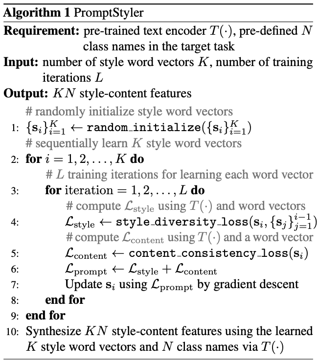
\[\mathcal{L}_{\text{prompt}} = \mathcal{L}_{\text{style}} + \mathcal{L}_{\text{content}} \tag{4}\]

위 loss를 활용한 학습 Algorithm 1은 다음과 같다.

2. Training a linear classifier using diverse styles

앞에서 학습한 $s_i$를 이용하여 Linear Classifier를 학습하는 과정이다.

1. $K$개의 style word vector $\lbrace s_i \rbrace_{i=1}^K$ 학습
2. $KN$개의 style-content feature 생성
   • 학습된 $K$개의 style word vector와 $N$개의 class를 이용
   • Text encoder $T(\cdot)$ 사용
3. Linear classifier 학습
   • $KN$개의 style-content feature과 class label을 사용

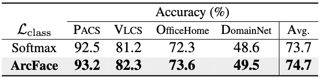
여기서 저자들은, Joint vision-language space를 활용하기 위해 ArcFace loss를 사용한다고 한다.

ArcFace loss란?

ArcFace는 얼굴 인식 작업을 위해 고안된 각도 기반 softmax loss function이다.

Classifier의 input feature와 가중치 간의 cosine 유사도를 계산하고 class 간 추가적인 각도 margin penalty를 적용한다.

\[L_{ArcFace} = -\frac{1}{N} \sum_{i=1}^N \log \frac{e^{s(\cos(\theta_{y_i} + m))}}{e^{s(\cos(\theta_{y_i} + m))} + \sum_{j=1, j\neq y_i}^n e^{s\cos(\theta_j)}}\]

각도 기반이기 때문에 Class 간 경계를 더 잘 형성하고 유클리드 거리 기반 손실 함수의 한계를 극복하기 위해 제안된 loss이다.

3. Inference using the trained classifier

학습된 Classifier를 Image Encoder $I(\cdot)$과 함께 Inference하는 과정이다.

1. vision-language space에 mapping된 Image feature $I(\text{x}) \in \mathbb{R}^C$를 추출
   • $\textbf{x}$는 Input image
   • Encoder $I(\cdot)$에서 이미지를 $\mathcal{l} _2$ 정규화
2. Classifer로 Class score를 생성
   • 위 image feature $I(\text{x})$를 사용

Experiments

Evaluation datasets

Generalization 성능을 평가하기 위해, 데이터셋이 아닌 4가지 Domain Generalization benchmark를 사용한다.

• PACS (4개의 도메인과 7개의 클래스)
• VLCS (4개의 도메인과 5개의 클래스)
• OfficeHome (4개의 도메인과 65개의 클래스)
• DomainNet (6개의 도메인과 345개의 클래스)

Implementation details

저자들은 RTX 3090 GPU에서 30분간 학습시키는 조건을 모두 동일하게 사용하였다고 한다.

Architecture

pretrained Vision-Language 모델로 CLIP을 사용하였으며, Image Encoder $I(\cdot)$는 ResNet-50을, Text encoder $T(\cdot)$는 Tramsformer를 사용하였다.

Image Encoder는 추가적인 비교를 위해 Vision Trasformer인 ViT-L, Vit-B도 사용

Learning style word vectors $s_i$

저자들은 $s_i$를 학습할 때, 다음과 같은 2가지 prompt learning 기법을 사용하였다고 한다.

1. Learning to Prompt for Vision-Language Models
   • 거대 Vision-Language 모델인 CLIP을 전체 fine-tuning하는 것은 비효율적
   • prompt를 도입하면 성능 향상에 효과적이지만 prompt engineering은 많은 시행착오가 필수적
   • Context Optimization (CoOp)를 도입하여 learnable vector 가 있는 prompt 의 context words 를 모델링
2. Conditional Prompt Learning for Vision-Language Models
   • 학습용으로 label이 지정된 이미지 몇 개만 사용하는 CoOp는 학습되지 않은 class로 일반화 불가능
   • conditional prompt learning를 도입하여 Input image에 따라 condition이 지정된 prompt를 만듬
   • 각 instance에 adaption되므로 class shift에 덜 민감하며, CoOp보다 domain generalization 성능이 향상됨

style word vectors $s_i$학습 조건은 다음과 같다.

• $\sigma = 0.02$인 zero-mean Gaussian 분포를 사용하여 $\lbrace s_i \rbrace_{i=1}^K$를 랜덤으로 초기화
• SGD optimizer : learning rate = 0.002, momentum = 0.9
• Total iteration = 100

Training a linear classifier

• 50 epochs
• SGD Optimizer : learning rate = 0.005, momentum = 0.9, batch size = 128
• ArcFace : scaling factor = 0, 각도 margin = 5

Inference

Input 이미지는 $224 \times 224$로 resize하고, 정규화를 진행하였다.

Evaluations

Main Result

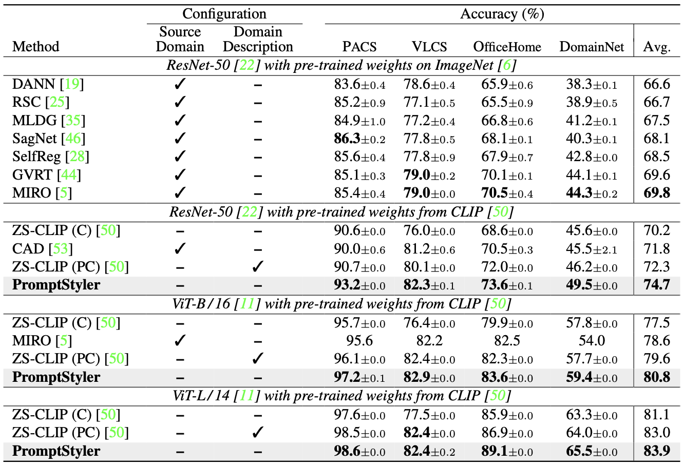
위 표를 보면 PromptStyler가 모든 benchmark에서 SOTA를 달성한 것을 알 수 있다.

zero-shot CLIP을 제외한 기존 방법들은 source domain 데이터셋을 사용하였으며, zero-shot CLIP에서 사용한

1. domain과 상관없는 prompt (“[class]”)
2. domain별 prompt (“a photo of a [class]”)

위 2가지 경우에도 PromptStyler가 더 좋은 성능을 보인다.

즉, latent space에서 prompt를 통해 다양한 분포 변화를 시뮬레이션함으로써 이미지를 사용하지 않고도 CLIP의 일반화 능력을 효과적으로 향상시킴을 알 수 있다.

**Computational evaluations. **

이 섹션에서는 parameter 수와 inference 속도를 비교한다. 비교 대상은 zero-shot CLIP과 PromptStyler이며, batch size를 1로 설정하고 단일 RTX 3090 GPU를 사용하였다.

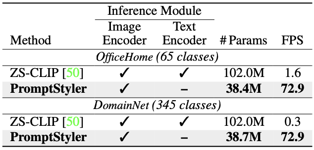
PromptStyler는 inference할 때 Text Encoder를 사용하지않아 zero-shot CLIP에 보다 가볍고 빠르다는 것을 알 수 있다.

t-SNE visualization results

prompt loss에 사용된 $\mathcal{L}_{\text{style}}$과 $\mathcal{L}_{\text{content}}$의 성능을 VLCS benchmark를 통해 평가하고, t-SNE로 시각화한다.

Visualizing Data using t-SNE

t-SNE는 t-SNE는 2차원 또는 3차원 지도에 가지고 있는 데이터 포인트에 위치를 부여함으로서 이를 시각화할 수 있도록 해주는 방법론이다.

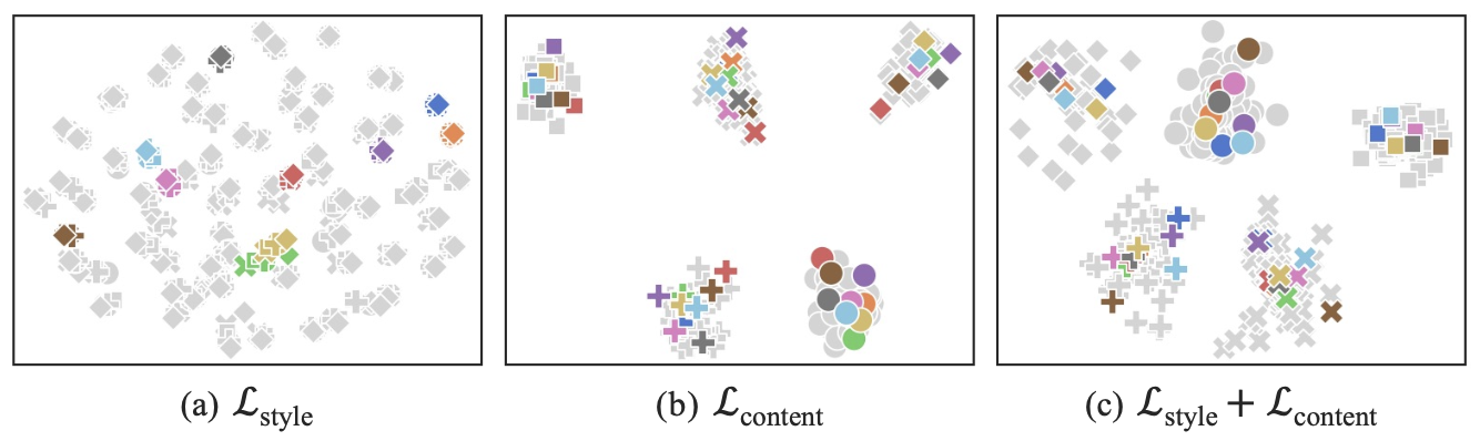
• (a) - $\mathcal{L}_{\text{style}}$ : 다른 class label(다른 모양들)과 유사한 feature를 공유(같은 색끼리 모여있음)

• (b) - $\mathcal{L}_{\text{content}}$ : style-content feature의 다양성 하락
• (c) - $\mathcal{L}_{\text{style}} + \mathcal{L}_{\text{content}}$ : content 정보를 왜곡시키지 않으면서 다양한 스타일을 생성

Text-to-Image synthesis results

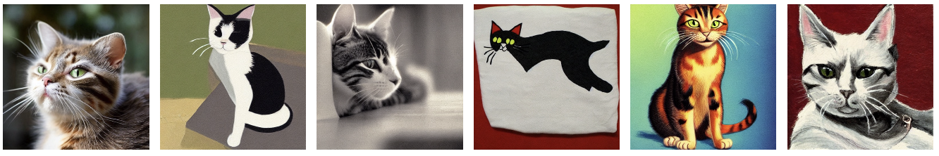
위 사진은 “a $\mathit{S}_{\boldsymbol{\ast}}$ style of a cat“에서 추출된 style-content feature를 diffusers라는 라이브러리로 시각화한시킨 결과이다. 6개의 학습된 style word vector $s_i$를 사용하였다.

More analyses

Loss

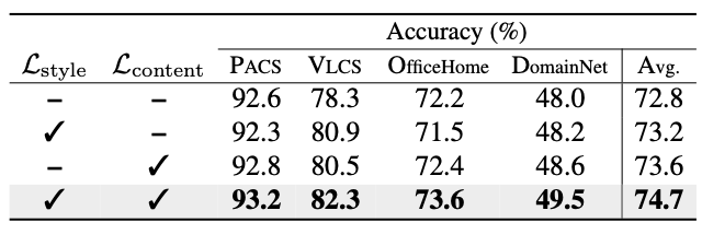
• 왼쪽 : Prompt Loss에 사용한 $\mathcal{L}_{\text{style}}$과 $\mathcal{L}_{\text{content}}$의 성능
• 오른쪽 : Classifier에 사용한 ArcFace Loss의 성능

Effect of the number of styles

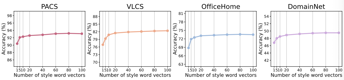
style 개수가 5개이상만 되어도 상당한 성능 향상을 보여준다.

**Effect of the number of iterations **

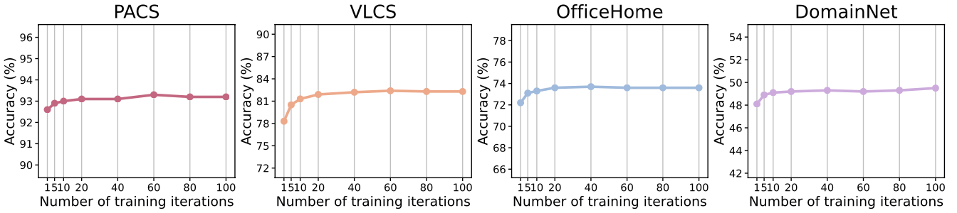
iter가 20번이면 충분히 좋은 결과를 얻을 수 있음을 알 수 있다.

Limitation

PromptStyler는 pretrained Vision-Language 모델의 joint vision-language space 성능에 의존한다. Terra Incognita 데이터셋의 경우, CLIP에서의 성능이 좋지 않기 때문에 PromptStyler에서도 성능이 감소하는 것을 확인하였다고 한다.

Code

Colab